The Nucleon Axial Coupling
Nature, DOI:10.1038/s41586-018-0161-8
My collaborators and I are glad to announce that the Standard Model of particle physics predicts that , the axial coupling of the nucleon, is 1.271±0.013. The experimentally measured value is 1.2723±0.0023.
Introduction
Motivation
Why do we need computers?
Wielding Lattice QCD to Calculate
Methodological Improvements
Outlook
Acknowledgements
Press Releases and Mentions
Introduction
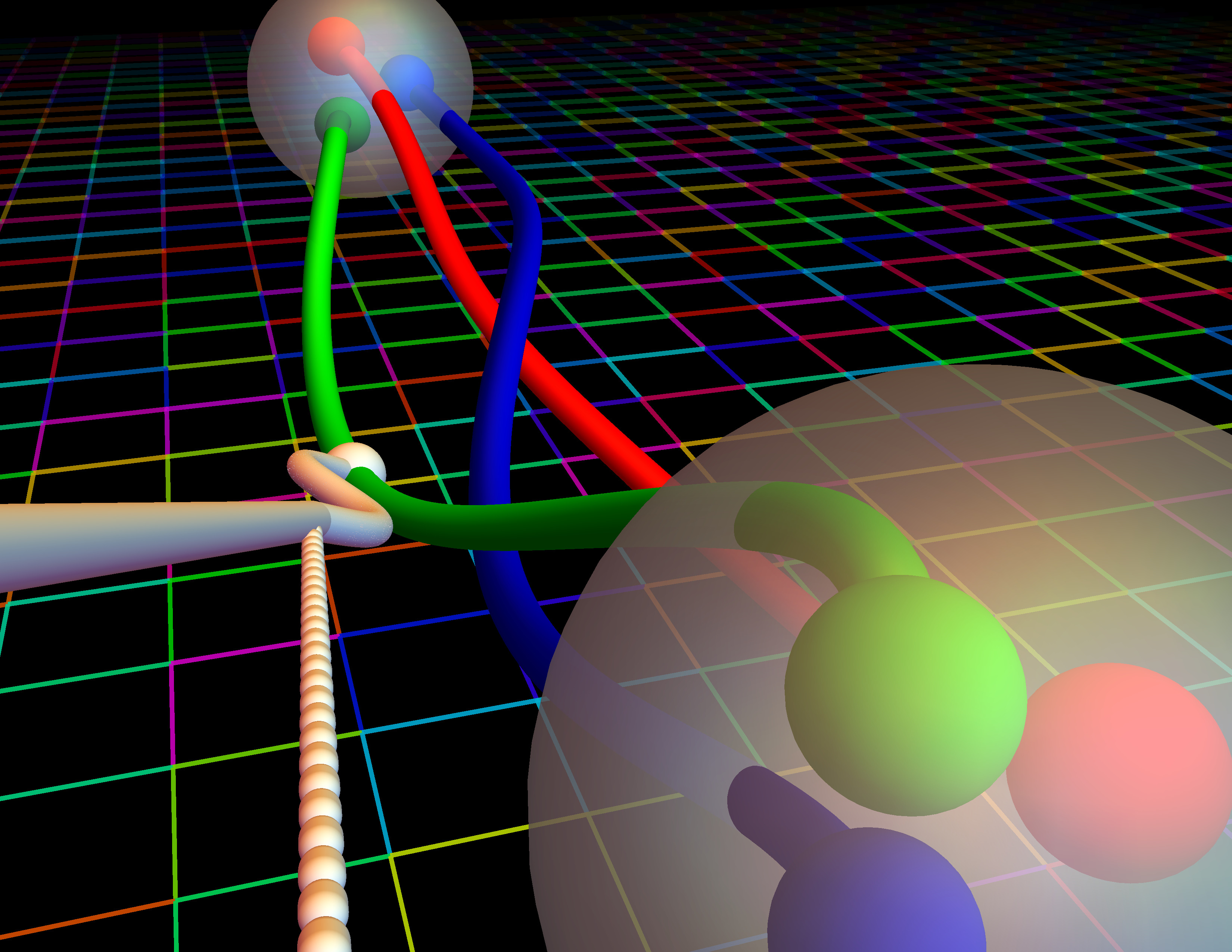
Protons and neutrons, collectively known as nucleons, are the particles that compose atomic nuclei. Nucleons, in turn, are made out of quarks and gluons, particles which are dominantly governed by quantum chromodynamics (QCD) and—as far as we know—are fundamental. Nucleons are baryons, and thus contain three “valence” quarks in addition to a big roiling mess of gluons and quark-antiquark pairs. Protons have two valence up quarks and one valence down quark, while neutrons have two valence down quarks and one valence up quark.
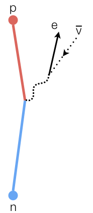
A free neutron decays into a proton, an electron, and an antineutrino.
The proton’s mass is 938.2 MeV, while the neutron’s mass is 939.6 MeV. That slight imbalance means that, by itself, a neutron can β-decay into a proton, an electron, and an antineutrino. But the rate of that decay isn’t controlled only by the masses involved. The decay rate also depends on the nucleon axial coupling, For experts, the axial coupling controls the Gamow-Teller transitions. . In the same way that electrons and protons have familiar electric charges which dictate how strongly they feel the influence of the electromagnetic interaction, nucleons have a charge, or coupling which dictates how strongly they feel the influence of the weak nuclear force, which causes β-decay, but also dictates how strongly they feel the influence of pions, which are the composite particles made of a quark-antiquark pair that bind nucleons into a nucleus.
Since nucleons are composite particles, this coupling can be determined by understanding the behavior of its constituents. However, unlike electric charge, which is conserved, determining the axial coupling of a neutron isn’t as simple as summing up properties of its valence quarks.
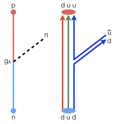
The nucleon coupling to the pion, drawn in the language of pions and nucleons and as the behavior of valence quarks.
You might wonder: if nucleons are composite objects without sharp edges, is there even any meaningful sense in which this coupling can be defined? Interestingly, the answer is yes. When trying to describe nuclear physics, we can write down a theory of pions and nucleons with all the same symmetries as QCD but which doesn’t talk about quarks and gluons any more. Matching the symmetries ensures we can force these theories to make the same predictions.
The cost of changing our picture is the introduction of a variety of unknown parametersThese unknown parameters are called low energy constants, or LECs, in the parlance of effective field theory. . That is, symmetry is strong enough to dictate the form of the theory, but isn’t enough to quantitatively match the two together. But, in principle, if we know enough about the underlying behavior of quarks and gluons we can match the two theories’ predictions to determine these numbers. Put another way, in the Cosmic Control Booth, God doesn’t have a dial that controls these numbers independently: she sets only the parameters of the fundamental theory, and all else is consequence.
Once determined, these parameters can be used to make predictions about the nuclear interaction. These numbers can be measured experimentally. Indeed, is known experimentally to be 1.2723±0.0023. These numbers can also be determined theoretically. We found that the underlying theory of quarks and gluons predicts 1.271±0.013.
Introduction
Motivation
Why do we need computers?
Wielding Lattice QCD to Calculate
Methodological Improvements
Outlook
Acknowledgements
Press Releases and Mentions
Motivation
If can be determined experimentally with better precision, why bother calculating it in the first place? The answer is three-fold.
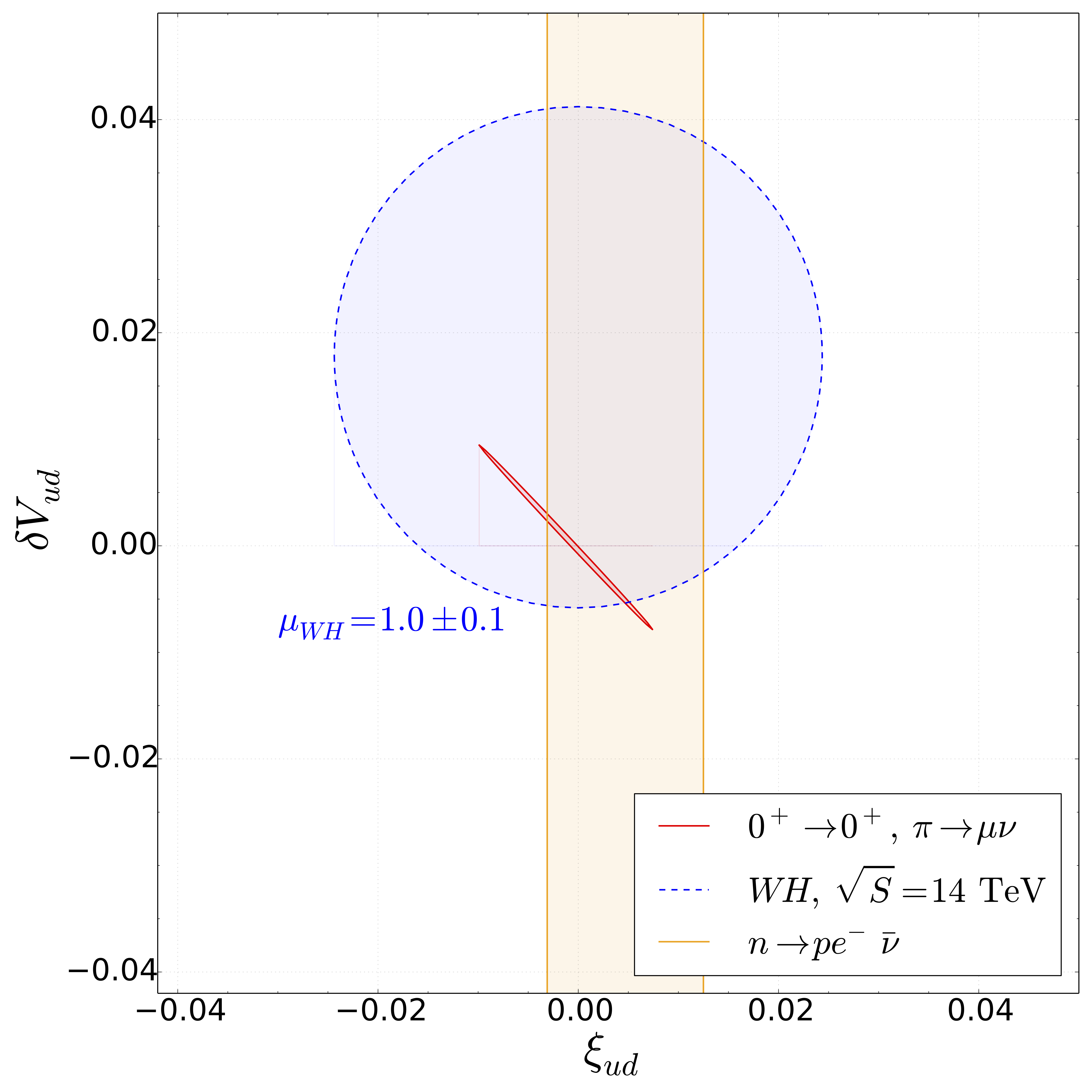
Colleagues generously provided us with this updated version of their Figure 12, showing three constraints on model-independent parameters that characterize new physics. The red ellipse comes from muonic pion decays, the blue circle from LHC W+Higgs production data, and the orange band is controlled by our result.
First, we want to make sure that the measured quantity is what it ought to be, assuming the Standard Model. If there were some new physics that modified this quantity, its effects would show up in experiments. But, in our calculations, we work only with physics described in the Standard Model. So, if there were a significant difference, it could be an exciting sign of new physics. That our result so closely matches what is found experimentally places tight limits on right-handed beyond-the-Standard-Model currents.
Second, we want to stress-test our calculating methods. Computing isn’t so straightforward, as I’ll explain below. In the future we will calculate quantities that aren’t measured well by experiment yet, and knowing we have our calculation under control will prove important. Having a benchmark quantity is a useful check that we know what we’re doing. The axial coupling is in some sense the simplest quantity in a larger set of observables, so it’s a good testbed for making sure we know where all the bodies are buried.
Finally, we like the laws of physics to be as unified a whole as possible. In principle, all of nuclear physics, from the simplest nuclei to neutron stars, should have a single, far-reaching description that originates in fundamental particle physics. While the method of summarizing the theory of quarks and gluons into a theory of nucleons and pions is perfectly well justified, as mentioned it comes with a cost of new, unknown parameters. Without calculation, these new parameters break the quantitative foundation of nuclear physics in particle physics. Computing the nucleon axial coupling is the first step in forging a quantitative connection that anchors nuclear physics in the underlying particle physics and reduces the number of input parameters one needs when describing physics as a whole.
Introduction
Motivation
Why do we need computers?
Wielding Lattice QCD to Calculate
Methodological Improvements
Outlook
Acknowledgements
Press Releases and Mentions
Why Do We Need Computers?
In many circumstances, when we want to extract information from a physical theory, we can use the following perturbative strategy:
- Make a good approximation to the answer, and get an answer that is accurate but approximate.
- Fix up the approximation, yielding a more daunting calculation, but improving the precision of the answer.
- Make ever-better approximations, undertaking ever more daunting calculations, and achieving better and better precision.
The theory of quantum electromagnetism is a theory where this strategy has enormous success, because there is a small parameter, the fine structure constant α, which is very small—about 1/137For experts, the perturbative expansion in quantum electrodynamics, and in most field theories, is thought to be an asymptotic expansion. . When we execute the above improvement scheme, the difference between each generation of results keeps getting smaller by factors of α. So, if you know to what precision you need your answer, I can tell you just how hard you need to work, in terms of how many times you have to go and fix up your approximation. Unless your problem is extraordinarily simple or has astounding mathematical properties, this fix-it-up strategy is the usual approach for pen-and-paper calculations.
The analogous number for QCD is about 1.5—a disaster for this perturbative method! Suppose you’ve worked very hard and made the third-least-stupid approximation. How many digits of accuracy can you expect? None, because there’s no sense in which the corrections get smaller and smaller. If you would only go and make the fourth-least-stupid approximation, you’d find your answer changes dramatically: your current result might even have the wrong sign. So you go and fix up your approximation further. How hard must you work to achieve a particular reliability? Hopefully it’s clear that with this perturbative strategy you can never stop and trust your result—the next piece will always dominate the answer and the work you’ve done so far is largely irrelevant.
Because this strategy fails, we call QCD a strongly interacting, or nonperturbative theory. Interestingly, QCD becomes perturbative at high energies, such as those found in colliders, where it has been tested vigorously and yielded predictions crucial for eliminating known signals from experiments and discovering new physics. To avoid this runaway disaster, we need a different strategy. We put QCD on a computer, and try to solve the whole thing without making any uncontrollable approximations. It could be that tomorrow someone has a new insight that allows us to solve QCD without computers. But the above argument about the failure of perturbation theory gives us a ‘folk theorem’ that no tractable pen-and-paper solutions exist.
Wielding Lattice QCD to Calculate
Introduction
Motivation
Why do we need computers?
Wielding Lattice QCD to Calculate
Methodological Improvements
Outlook
Acknowledgements
Press Releases and Mentions
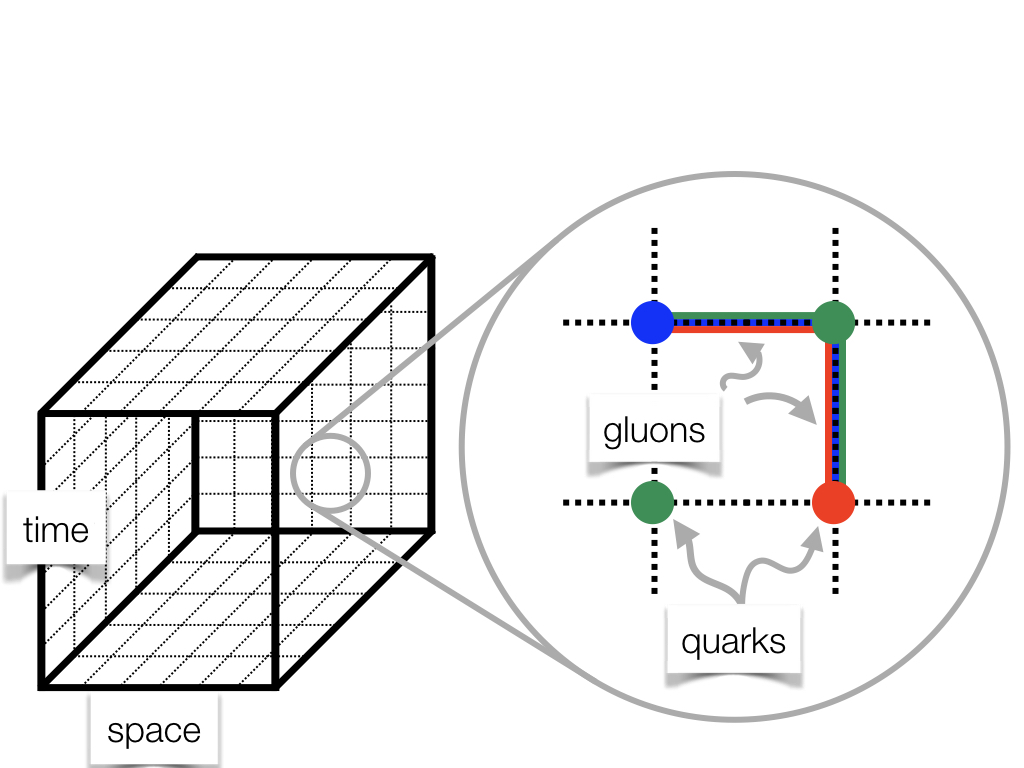
A cartoon of a four-dimension lattice used in lattice QCD. The interior sites and links have been omitted for clarity.
Lattice QCD is the formulation of QCD on a finite, discrete spacetime. This transforms the problem from a horrible infinite-dimensional integral to a still-horrible but finite-dimensional integral, which we attempt to evaluate via importance sampling Monte Carlo methods.
Typically we use a square lattice, but in four dimensions. We put the quarks on sites—the intersections of the grid—and the gluons on links—the lines that connect the sites. The gluons determine how the quarks can move around, and so naturally live on the connections between sites. We have to sample many different possible configurations—arrangements of fields in spacetime—to correctly capture the quantum-mechanical properties. The more configurations we can sample, the better our answer. We generate these configurations with a Markov chain, and each configuration is computationally expensive to create. In other words, if someone is willing to pay the electric bill, we can drive down the uncertainty on our answer further and further, but it ain’t cheap.
The day-to-day activities of a lattice QCD practitioner look a lot like an experimentalist—there’s statistical data analysis, curve fitting, and understanding and quantifying uncertainties. We often refer to the quantities we compute on each configuration as “measurements”—although of course we’re aware that we’re not poking and prodding Nature itself. Instead, just as a telescope lets you see deep into space, a computer lets you see deep into the Platonic mathematical realm. At the end, we quote an answer with a controlled uncertainty that accounts for both the statistical nature of the approach, and any systematic difficulties, just as an experimentalist might.
There are three standard sources of systematic uncertainty in lattice QCD which must be addressed. Obviously, we use a discrete spacetime even though we are interested in the continuum. Although we’re interested in physics in an infinite spacetime volume, we use only a finite spacetime volume so that our problem fits in a finite-size computer memory and our calculations finish in a finite amount of time. We have another trick as well: we can change the parameters of QCD! So, the computational physicist can answer questions the experimental physicist cannot, such as what would happen if one could adjust the dials in the Cosmic Control Booth that are impossible to adjust experimentally. Experimentalists are stuck with the true values—we have to make sure we can ultimately get to the experimental values.
At short distances, QCD is perturbative and we know the exact theory we are interested in. That means we can take our lattice spacing—the length of the links—finer and finer so as to match QCD, and then let the computer handle the long-distance, nonperturbative mess. We calculated at three lattice spacings: 0.15, 0.12, and 0.09 fm1 fm, a femtometer, or fermi, is 0.000000000000001 meters. A proton is about 1 fm across. and extrapolated to the continuum limit. We avoid going to ultrafine lattices because the numerical cost grows quickly as the lattice spacing shrinks.
Of course, the computational cost also grows with the number of sites in each direction, yet we want to make sure our calculations aren’t too badly distorted by being in a finite volume. One helpful technique is to use periodic boundary conditions—like in Pac-Man—to ensure the lattice has no edges or walls and no site is privileged to be in “the middle”. Still, we calculated at a variety of different volumes, making sure to carefully take the infinite-volume limit.
Finally, for technical reasons, some numerical steps become very expensive as the quark masses get close to zero.This growth in cost is caused by the Dirac operator becoming more-and-more ill conditioned. Multigrid methods alleviate this problem. In nature, the up and down quark masses are just a few MeV while the natural scale of QCD is a few hundred MeV (for example, the proton and neutron masses, as mentioned, are about 940 MeV) and in this sense are very small; only in the last 10 years or so have calculations with physical parameters been achieved. We calculated on five quark masses from 130 MeV to 400 MeV, allowing us to interpolate to the near-physical pion mass of about 138 MeV.
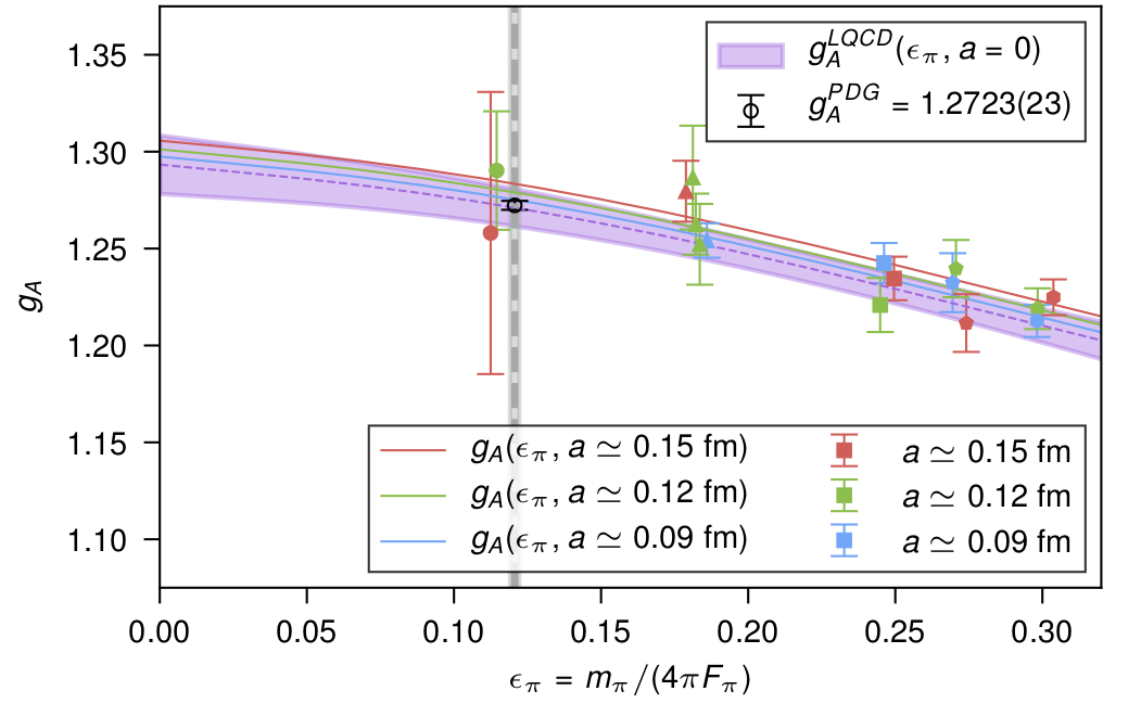
By calculating at three different lattice spacings, different volumes, and different quark masses, we control all three sources of systematic uncertainty and recover a function (and its uncertainty band) that describes the axial coupling as a function of the pion mass in the continuum and in infinite volume. Our final quoted result
is the value of that function at the physical pion mass, the error accounting for statistical uncertainties, uncertainties from interpolating/extrapolating to the physical parameters of QCD, to the continuum, to an infinite volume, from omitting the small mass splitting between up and down quarks, and from fitting.
Introduction
Motivation
Why do we need computers?
Wielding Lattice QCD to Calculate
Methodological Improvements
Outlook
Acknowledgements
Press Releases and Mentions
Methodological Improvements
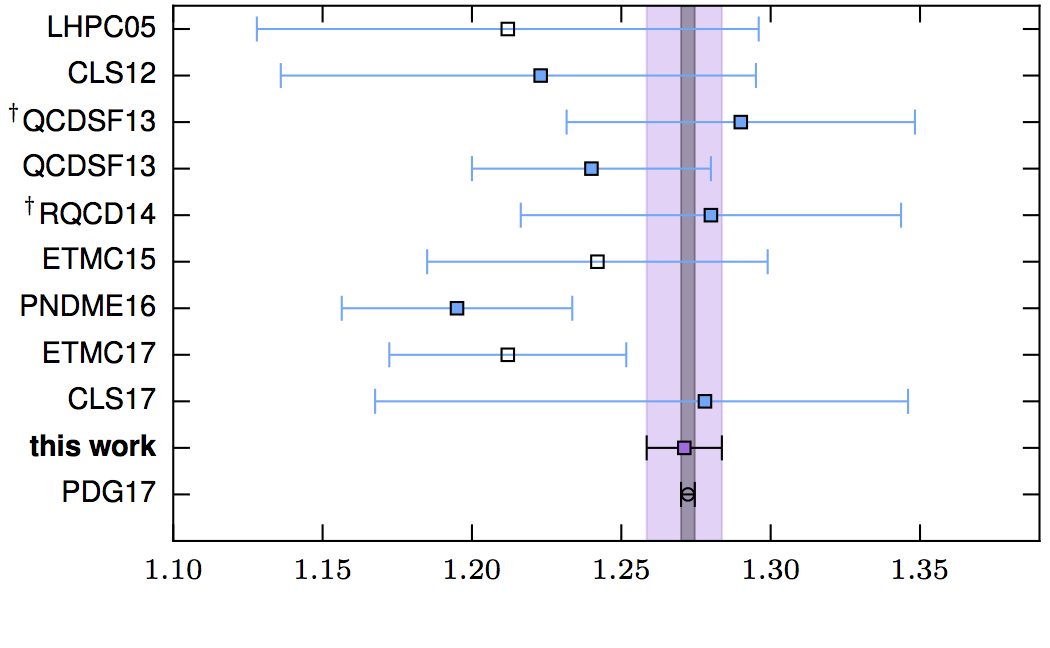
A comparison of previous calculations, our result (purple, with an error band to guide the eye), and the experimental determination given in the PDG.
We are by no means the first group to compute the nucleon axial coupling using lattice QCD. However, the 1% uncertainty we achieved is an enormous improvement over previous results. This marked improvement wasn’t simply a matter of using a larger amount of computer time, but relied on new methods. In fact, people expected that a 2% uncertainty would be achieved by 2020, possible only with the next generation of supercomputers. It’s natural to ask: what did we do differently that unlocked this precision result?
The quantities we need to determine are correlation functions, which tell you how quantities change across the spacetime volume. In particular, we need to know the long-time behavior of those functions. Unfortunately calculations with baryons have an exponentially-bad-in-time signal-to-noise problem, which means that the later we look in time the larger the statistical fluctuations are and so the less reliable the measurements are. One expensive way to overcome this problem is through sheer strength, overcoming this difficulty with ever-increasing statistics.If you know a funding agency with an exponentially large computer or an exponentially large budget, point me their way! Previous calculations focus on a few values of these functions, at just a few intermediate and late times, hoping to get a good signal that still captured the late-time behavior without breaking the bank.
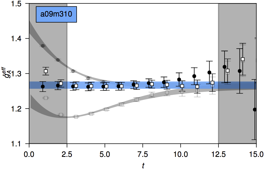
Instead, we use a different method to determine these functions, which, for the same computational cost as a single point, gives us access to the functions at all times. The benefit of this approach is that it yields access to points at early times which are exponentially better in terms of a signal-to-noise precision. While these early-time points don’t accurately capture the late-time behavior, knowledge of how these functions evolve in time allow us to fit and make a reliable late-time extrapolation. The drawback of this method is that we only have access to the axial coupling in this calculation, while the more common method yields access to many different nucleon properties; we can compute these other properties, but at additional cost.
The clear reliability of our late-time extrapolation depends on computing these functions at all times, and leveraging the precision of the early times, where the noise isn’t bad.
Introduction
Motivation
Why do we need computers?
Wielding Lattice QCD to Calculate
Methodological Improvements
Outlook
Acknowledgements
Press Releases and Mentions
Outlook
With this determination of the axial coupling, we have demonstrated the potency of lattice QCD for nuclear physics. But, this is by no means the end of the story—indeed, it is just the beginning. There are many interesting single-nucleon properties important for translating experimental results into knowledge of new physics. The hunt for exotic, ultra-rare processes, such as neutrinoless double beta decay, requires quantitatively connecting very high energy particle physics with very low energy nuclear physics with controlled errors, and lattice results will form an important link in that chain of evidence. Ultimately, a quantitative understanding of one-, two-, and other few-nucleon systems from lattice QCD will supplant phenomenological modeling as the basis of nuclear physics.
Acknowledgements
![]()
The computing power for the calculation was provided by the Department of Energy’s Innovative and Novel Computational Impact on Theory and Experiment (INCITE) program to CalLat (2016) as well as by Lawrence Livermore National Laboratory (LLNL) Multiprogrammatic and Institutional Computing program through a Tier 1 Grand Challenge award.
We used Titan, an NVIDIA GPU-accelerated supercomputer, at the Oak Ridge National Laboratory, which is supported by the Office of Science of the U.S. Department of Energy under Contract No. DE-AC05-00OR22725, and the GPU-enabled Surface and RZHasGPU and BG/Q Vulcan clusters at LLNL.
As explained, lattice QCD calculations are performed with Monte Carlo ensembles of field configurations. Most of the ensembles we used were produced by the MILC Collaboration, though we generated some of our own as well.
![]()
![]()
![]()
![]()
We were supported by our employers and funding agencies, NVIDIA, the DFG and NSFC Sino-German CRC 110, Lawrence Livermore and Lawrence Berkeley National Laboratories’ Lab Directed Research and Development (LDRD) programs, the RIKEN Special Postdoctoral Researcher Program, the Leverhulme Trust, the Department of Energy Offices of Science’s Nuclear Physics, Advanced Scientific Computing Research, SciDAC and Early Career Research programs, as well as through its Nuclear Theory for Double Beta Decay and Fundamental Symmetries Topical Collaboration.
We had helpful input on our work, in its various stages, from C. Bernard, A. Bernstein, P.J. Bickel, C. Detar, A.X. El-Khadra, W. Haxton, Y. Hsia, V. Koch, A.S. Kronfeld, W.T. Lee, G.P. Lepage, E. Mereghetti, G. Miller, A.E. Raftery, D. Toussaint and F. Yuan.
Introduction
Motivation
Why do we need computers?
Wielding Lattice QCD to Calculate
Methodological Improvements
Acknowledgements
Press Releases and Mentions
Press Releases and Mentions
This list will be updated sporadically.
- Mikroskopisches Universum gibt Einblick in Leben und Tod des Neutrons [English translation]
- Supercomputers give scientists key insight into the lifetime of neutrons
- Simulations capture life and death of a neutron
- Supercomputers Provide New Window Into the Life and Death of a Neutron [UIUC Alumnus News]
- With Supercomputing Power and an Unconventional Strategy, Scientists Solve a Next-Generation Physics Problem
- Nuclear Scientists Calculate Value of Key Property that Drives Neutron Decay
- 中性子の寿命の仕組みを垣間見る
- New Physics Research Aims to Answer the Mysteries of the Universe
- Un quatro d’ora da neutrone
- Počítačové simulácie posúvajú hranice poznanie sveta
- The CalLat Collaboration have calculated the axial charge of the nucleon with an unprecedented one-percent precision
- Supercomputers provide new insight into the life and death of a neutron
- Rätselhafte Atombausteine